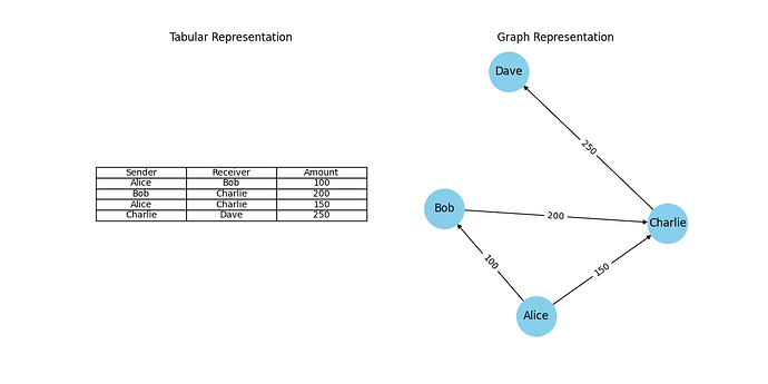
Right: The same data visualised as a network. Nodes represent people, and edges represent transactions. This structure makes it easier to detect patterns, such as loops or clusters, in the flow of money.
By Yiming Wu (Senior Data Scientist, Applied AI) and
Mihir Tare (Senior Machine Learning Engineer, Applied AI)
Large financial organisations process millions of transactions every day and each one tells a small story — who paid whom, when and how much. Analysing these interactions helps us uncover patterns across customer habits, business trends, signs of fraud and so on. In this blog, we will showcase how we used a unique network-based approach to unlock the potential of transactional data in the context of banking.
Traditional analytical methods often struggle to effectively leverage the information contained within these interactions. Using a classic tabular approach overlooks a key strength of this data as it fails to capture how people and businesses are connected. Here, transaction data is normally represented in a tabular format where each row represents a single transaction, containing attributes like sender, receiver, amount, time etc. Each transaction is treated as an independent event, which is efficient for storage and querying of the data, but fails to capture any relational structure within it. Traditional machine learning models rely on these structured datasets and struggle to leverage the connections between the rows.
We take a different approach to address this problem by utilising mathematical objects, called graphs, to analyse transaction networks. A graph is a mathematical structure used to represent information in the form of nodes and edges. Nodes are used to represent entities, like accounts or merchants, and edges are used to represent the connections between these nodes, like monetary transactions. In the world of financial analytics, the terms graphs and networks are often used interchangeably. By shifting from tabular to graphical representations, we can apply graph-based machine learning techniques that are better suited to uncovering hidden structures, community behaviour, and anomalies in transaction data.
Following the simple example above, we designed our population to construct a well-rounded graphical representation of all the interactions between the accounts on our transaction data.
The transaction network contains four types of nodes:
These 4 node types induce 7 types of edges on the graph which can be seen in the figure below. While the edge types are described individually, they all indicate the same underlying interaction on the network — a flow of money between two accounts — and are uniquely identifiable using the sender-receiver account types pair.

The resulting graph contained over 100 million transaction and over 10 million nodes.
Great, so now you have an intuitive way to visualise your transaction data on a graph, but how do we use this? This is one of the main challenges when it comes to using graph-based approaches in the world of machine learning. As most models use fixed-length tabular data as inputs, not graphs, we turn towards a special suite of models called Graph Neural Networks (GNNs). Using a GNN, we can do one of two things:
While the first is a viable option, the model is purpose built and commits to solving only one task using only the graph information. On the other hand, embeddings are a general-purpose, reusable asset containing summarised information about interactions on the graph. This allows us to use graph information in solving various problems, without any additional processing, alongside other useful data.
As noted earlier, large banks process millions of transactions every day. In order to train an embedding model for this massive network, your algorithm must be able to scale efficiently. We achieve this by adopting a sampling-based embedding algorithm known as GraphSAGE. GraphSAGE avoids processing the entire graph at once by sampling a small set of neighbouring nodes for each node during training. The sampled neighbourhood is passed to an information aggregator to compute embeddings for each node. This makes it possible to train on massive graphs without running into memory or time constraints.
In our implementation, we use a mean aggregator for computing the embeddings and sample neighbouring nodes uniformly at random. In addition to maintaining computational efficiency, the neighbourhood sampler also nullifies the impact of super-connected nodes, such as supermarkets with thousands of daily transactions, on the training duration.
As with training traditional neural networks, we had to use a loss function to optimise the trainable parameters of the model. Taking inspiration directly from the original publication of GraphSAGE [2], we implemented an unsupervised loss function which maximises the similarity in the embeddings of neighbouring nodes and minimises the similarity in the embeddings of non-neighbouring nodes. Here, the neighbouring nodes are obtained through the neighbourhood sampling stage and the non-neighbouring nodes are obtained using a negative sampling distribution. The negative samples are examples of nodes that are not connected on the graph and allow the model to learn what dissimilar accounts look like. This is done uniformly at random by sampling edges that do not exist on the transaction network. This part of the implementation is key for enabling the embeddings to be a reusable asset.
This three-stage algorithm enables the model parameters to be trained in mini-batches on GPU-enabled machines by using standard stochastic gradient descent and backpropagation. The model was trained on a graph containing over 100 million transactions using g5.16xlarge AWS EC2 instance in 4 hours and was able to run inference on a g5.8xlarge instance in under 20 minutes. The output embeddings from the model are 32-dimensional vectors and the hyperparameters were optimised based on empirical experiments that balanced model complexity and performance.
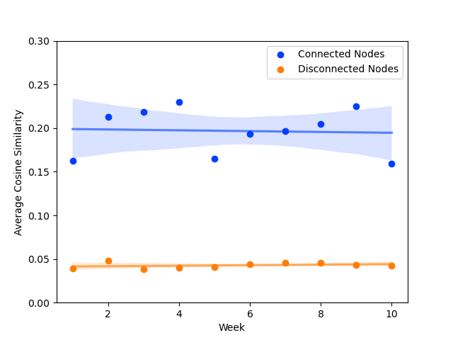
We trained our GraphSAGE model to compute 32-dimensional embeddings for all the accounts and merchants in our transaction network.These embeddings are compact numerical representations that capture the structure and behavior of each account based on its transactions on the network. At first glance, these embeddings are abstract pieces of information; vectors of numbers that don’t inherently “mean” anything in isolation. However, their power lies in how they relate to one another. Accounts that are structurally or behaviourally similar on the network will have embeddings that are close together in this high-dimensional embedding space.
To validate this claim, we computed the cosine similarity between embeddings of connected nodes (i.e. accounts that have transacted with each other) and compared them to disconnected nodes. The results showed a clear pattern: connected nodes had higher similarity scores on average, indicating that the embeddings successfully captured meaningful relationships from the transaction graph. This cosine similarity difference was an interpretable measure of how the unsupervised model was performing at its task. As a result, we used it as a lightweight metric to monitor the model performance in production, enabling us detect issues like model degradation.
While the cosine similarity difference was an effective quantitative measure of model performance, we explored some qualitative measures to visualise the embeddings and their quality. To interpret the deeper topological information captured embeddings, we used a Uniform Manifold Approximation and Projection (UMAP) model to project the embeddings to a lower, 2-dimensional space. The 2-dimensional projection allowed us to visualise the structure of the embedding space and observe how accounts naturally clustered based on their transactional behaviour.
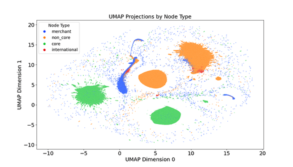
As seen in the image above, the initial investigation using UMAP revealed that the model was clearly able to understand the difference between the different types of nodes on the graph. Each cluster on the plot reflects a distinct pattern of interaction within the transaction network, potentially describing how routine spending, business flows, peer-to-peer transactions, or anomalies are separated when visualised this way. When the population was filtered to display only NatWest accounts, the UMAP plot revealed clusters clearly distinguishing current accounts from savings accounts as seen below.
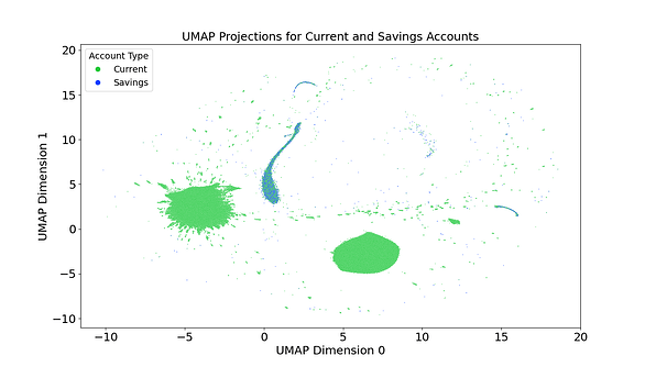
This revealed an unexpected similarity in behaviour between savings accounts merchants as they can only interact with current accounts.
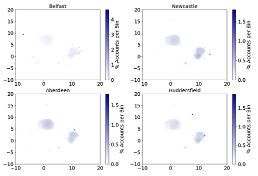
A deeper investigation into these UMAP projections exposed the model’s ability to capture geographical information of accounts. The next figure shows four density plots where the opacity of each pixel is determined by the number of accounts with their UMAP projection in that region.
Specifically, a darker a pixel indicates more accounts with a UMAP projection belonging to that region. For each plot, the population was filtered based on the postcode area of the branch (namely, in Belfast, Newcastle, Aberdeen and Huddersfield) that the accounts are registered with. The presence of distinctly dark pixels at unique locations in each plot showcases that geographical clustering is induced in the embeddings generated by this model. This is most clearly visible in the plot for Belfast showing over 4% of accounts clustered in the top left corner.
The presence of these geographical clusters could be attributed to two potential reasons:
The model’s ability to induce this information without any prior knowledge of the accounts’ locations, purely based on transaction activity, is a testament to its ability to capture topological information beyond just the connectedness of the network. This information is induced through the transactional behaviours of each account and can be a highly valuable proxy for account information to many downstream applications.
Note: UMAP is a dimensionality reduction algorithm and will inevitably not be able to represent all the information contained within the original 32-dimensional embeddings. Nonetheless, they still provide us with a very tangible evidence for the successful training of the model.
Because our model is trained in a completely unsupervised way, the embeddings it produces aren’t tied to any one task. This makes them incredibly versatile, allows them to be reused across a wide range of downstream applications that benefit from understanding transactional behaviour. To demonstrate this flexibility, we applied the embeddings to a real-world challenge: detecting money mules. Money mules are individuals who act as intermediaries between suspicious and legitimate accounts, often unknowingly helping to launder money. Identifying them is critical for banks, as they play a key role in concealing the origins of illicit funds and can face serious legal consequences themselves.
We tested the value of the embeddings by comparing two versions of a money mule detection model. The first used only traditional account-level features and served as our baseline. The second used the same features but added the 32-dimensional embeddings as additional inputs. We evaluated both models using two key metrics:
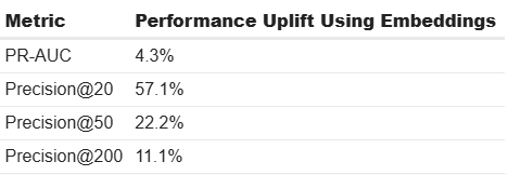
While we can’t share the raw numbers due to the sensitivity of the data, the results revealed that the model that included embeddings outperformed the baseline, especially in the top-ranked predictions. In fact, precision among the top 20 flagged accounts improved by 57.1%, a major win for fraud analysts who often have limited time and need to focus on the highest-risk cases.
Even though the overall PR-AUC did not change dramatically, this was likely due to the highly imbalanced nature of the dataset. However, it remained stable, confirming that the embeddings did not degrade performance. Instead, they sharpened the model’s ability to prioritise the most critical cases, highlighting their practical value in real-world fraud prevention.
One of the exciting aspects of our approach is that the model can infer fresh embeddings on a regular basis, we currently do this every week. Meaning, we are not just capturing a static snapshot of an account’s behaviour, but rather building a dynamic view of how its transactional neighbourhood evolves over time. Think of it this way: each week, the embedding reflects where an account “lives” in the transaction network during that time. By comparing its embeddings over time, we can understand how that account moves on this network as its behaviour shifts. This can indicate whether it becomes more active, connects with new types of entities, or starts to resemble known risky patterns. This opens the door to an interesting next step: a temporal analysis of embeddings. In financial services, behavioural changes over time are often more telling than static features. A customer who suddenly starts transacting with high-risk accounts or changes their spending patterns dramatically might warrant closer attention. Embeddings give us a compact, data-driven way to track and quantify these shifts.
This work also introduces some interesting challenges from a technical perspective. As the size of the transaction network grows, so does the computational demand. Implementing distributed training across multiple GPUs would significantly reduce training time and make it feasible to update embeddings more frequently or at larger scales. A more sophisticated implementation like this could also enable us to use these embeddings in real-time in the future.
The network remembers everything. The question is: what will you discover?
If you found our work interesting and would like to solve similar problems, we encourage you to take a look at our available job openings!
This work has been published in LNCS. For the full academic treatment, check out our paper on arXiv here.
[1] Self Supervised Learning for Graphs, Medium
[2] Inductive Representation Learning on Large Graphs, arXiv
<hr><p>The Geometry of Money: How we used Graph Neural Networks to transform financial network analysis was originally published in NatWest Group AI & Engineering on Medium, where people are continuing the conversation by highlighting and responding to this story.</p>